Experiment 37 Fiber Optics and Electro-Optical Characteristics of Semiconductor Laser
During the 1960s and 1970s, significant advancements were made in the realms of optical fiber communication and semiconductor laser technology. Optical fibers, acting as optical waveguides, boast a multitude of benefits for communication purposes, including substantial bandwidth capacity, minimal frequency loss, extended transmission ranges, and immunity to electromagnetic interference. Semiconductor lasers, known for their compact size, lightweight nature, high efficiency, and cost-effectiveness, serve as excellent electro-optical transducers. They are extensively utilized in various applications such as optical communication, data storage, optical gyroscopes, laser printing, distance measurement, and radar systems.
Figure 37-1 Approximate measurements of the NA of a fiber
Applications of optical fibers include:
- Communications - Voice, data, and video transmission are the most common uses of fiber optics, and these include:
- Telecommunications
- Local area networks (LANs)
- Industrial control systems
- Avionic systems
- Military command, control, and communications systems
- Sensing - Fiber optics can be used to deliver light from a remote source to a detector to obtain pressure, temperature, or spectral information. The fiber also can be used directly as a transducer to measure a number of environmental effects, such as strain, pressure, electrical resistance, and pH. Environmental changes affect the light intensity, phase and/or polarization in ways that can be detected at the other end of the fiber.
- Power Delivery - Optical fibers can deliver remarkably high levels of power for tasks such as laser cutting, welding, marking, and drilling.
- Illumination - A bundle of fibers gathered together with a light source at one end can illuminate areas that are difficult to reach — for example, inside the human body, in conjunction with an endoscope. Also, they can be used as a display sign or simply as decorative illumination.
Objectives
- Understand the basic structure of an optical fiber, and the electro-optical characteristics of semiconductor laser.
- Master the method to obtain the threshold current of a semiconductor laser by graphing method.
- Master the concepts and measurement methods of coupling efficiency and numerical aperture.
- Preliminary understanding of the principle of optical fiber communication technologies.
Instruments
GX1000 Optical Fiber Tester (including an Optical Receiver), Optical Fiber, Semiconductor Laser, Long Linear Optical Guide Rail, OPT-1A Laser Power Meter (including a Detector Head), Short Linear Displacement Rack, Sound Source (Provide Yourself), Bearing Rods and Clips, Signal Wires, etc.
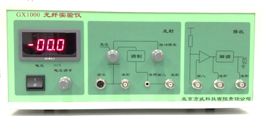
Figure 37-1 Approximate measurements of the NA of a fiber
Principle
1. Electro-Optic Characteristics of a Semiconductor Laser
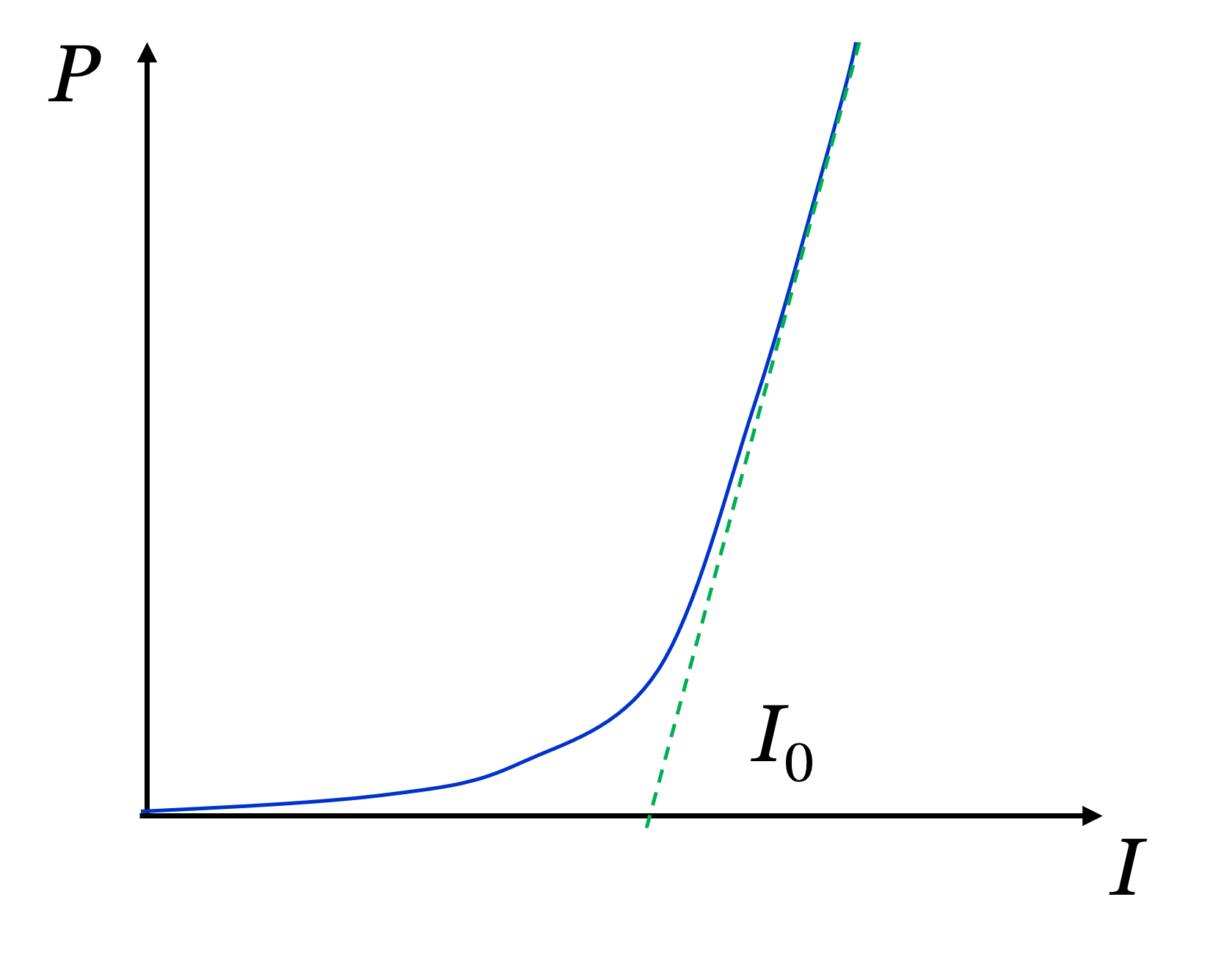
Figure 37-1 Characteristic Curve of a Semiconductor Laser
When the driving current I of a semiconductor laser is less than a certain value, the output optical power of the emitting light is very small, and no laser beam is obtained. When \(I\) is greater than the threshold current \(I_{0}\) , the output optical power increases rapidly and the emitting light becomes a laser beam. The relationship between the drive current and optical output power for a semiconductor laser is called electro-optical characteristics. A typical characteristic curve is shown in Figure 37-1.
2. Optical Fiber’s Structure
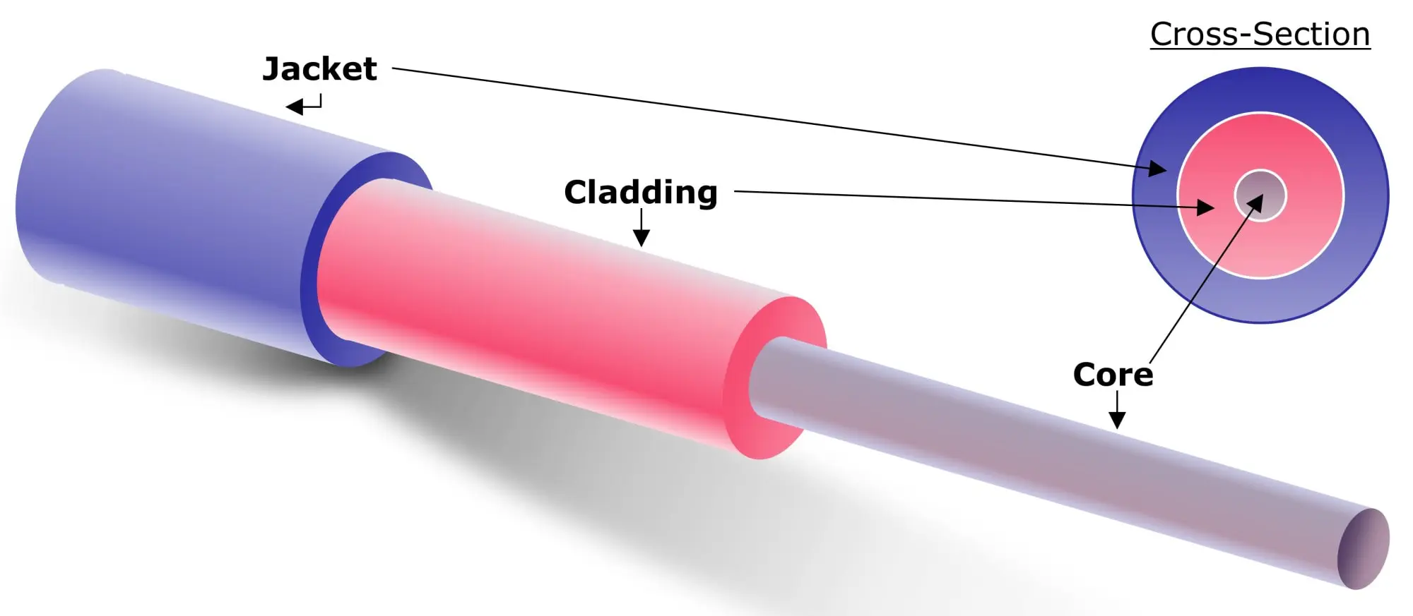
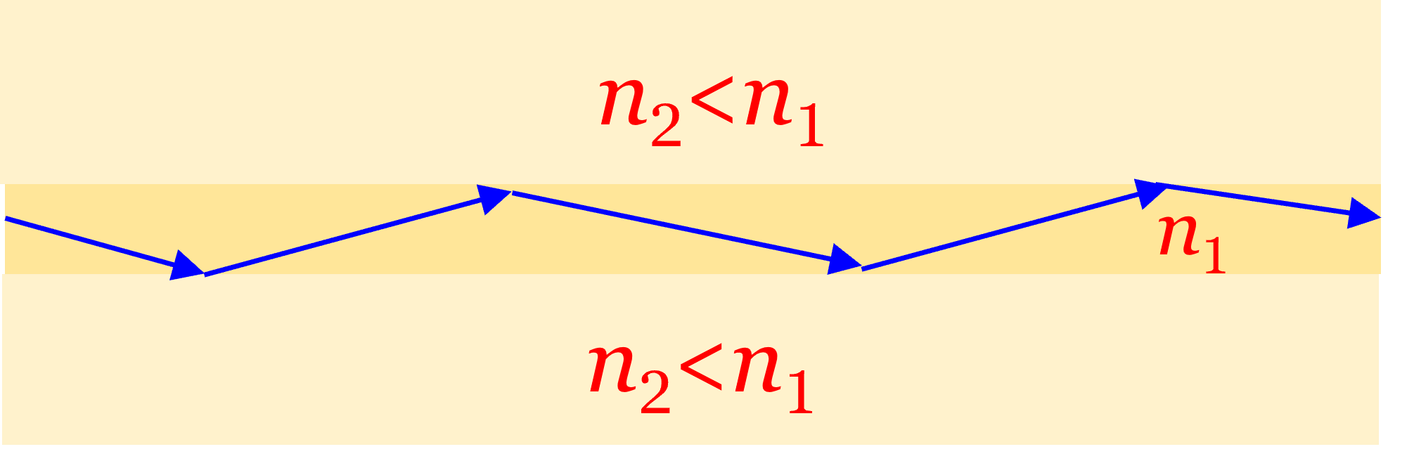
Figure 37-2 Typical Structure of A Step-index Fiber
As shown in Figure 37-2, A step-index fiber is a cylindrical dielectric waveguide specified by its core and cladding refractive indices, \( n_{1}\) and \( n_{2}\). It usually has a three-layer structure with a core, a cladding layer, and a coating layer (protective layer). The core and cladding layer are all made of quartz glass. In order to form a total reflection condition between the core and the cladding layer when a light beam travelling in the optical fiber, the refractive index in the core is a little larger than that in the cladding layer, and the light travels mainly in the core.
3. Optical Fiber-Laser Beam Coupling
The coupling between the optical fiber and laser beam can occur on the input end face of the optical fiber, and then the laser beam can enter and travel along it. The coupling quality can be judged from the intensity of output light spot from the other end of the optical fiber.
Coupling Efficiency \( \eta\) indicates the ratio of optical powers that enters the fiber (\( P_{1}\)) to the source’s (\( P_{0}\)):
$$ \tag{37-1}\eta =\frac{P_{1}}{P_{0}} \times 100\%$$
4. Numerical aperture
Numerical aperture NA describes the light-gathering capacity of an optical fiber. It can be estimated by measuring the distribution of optical power at the fiber’s output side. A quick approximate measure of the fiber's NA can be get using the image formed on a piece of paper placed a distance \(l\) away from the output end of the fiber in a darkened room, as shown in Figure 32-3. Measure the radius \(r_0\) of the spot and the distance l between the fiber end and the card. The NA of the fiber is approximately
$$\tag{37-2}\mathrm{NA} =\sin \left [ \tan^{-1} \left ( \frac{r_0}{l} \right ) \right ]$$
\(r_0\) also can be obtained using an optical power meter with a movable detector head. The full width of the output spot therefore is determined from the \( P-r\) curve that measured along the radial direction of the output spot. The edge of the spot is stipulated at the points where the received power is at \( \frac{1}{e^2}\) or 5% of the maximum intensity.
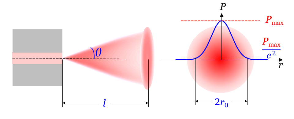
Figure 37-3 Approximate measurements of the NA of a fiber
5. Optical Fiber Communication
As shown in Figure 37-4, general processes of optical fiber communication are:
- Load the information (language, image, text, data) onto the optical carrier in optical transmitter;
- Couple the information-carrying light into the fiber core;
- Transmitted information-carrying light to optical receiver via optical fiber;
- Optical receiver processes (amplifies, decodes, and shapes) the received signal, and then restores the original transmitted information (language, image, text, data).
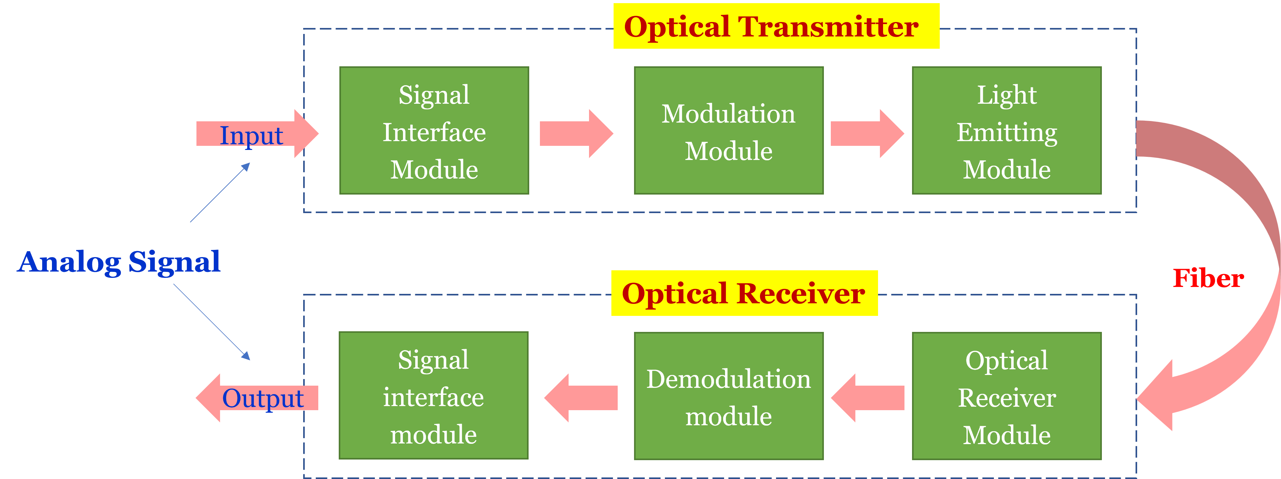
Figure 37-4 Approximate Measurements of the NA of a Fiber
Content and Procedure
1. Familiar with experimental instruments
Figure 37-5 is a schematic diagram of the experimental process. The GX1000 optical fiber tester is the experimental host that supplies power to the semiconductor laser via the transmit module and power module. Laser light from the semiconductor laser is coupled into the fiber from the input end face of the it. After a length of fiber transmission, the light ejects from the output end face of the fiber. Different optical transducer will convert the output laser signal into needed forms. For example, if the transducer is a detector head connected with OPT-1A Laser Power Meter, we can get the optical power of the output light.
2. Preparation Work
- Turn on OPT-1A Laser Power Meter, adjust the “Range Adjustment” knob to the 2mW, and zero the power indicator without laser irradiation.
- Place the “Function Selector” knob of GX1000 Optical Fiber Tester on “DC” position, and rotate the “Current Adjustment” knob counterclockwise in the power module to the minimum. Turn on the host.
3. Fiber-Laser Coupling and Coupling Efficiency Measurement
- Move the sliding blocks of the fiber and semiconductor laser so that the distance between the input end of the fiber and the laser is kept at about 20 cm.
- Slowly rotate the “Current Adjustment” knob clockwise to make the laser drive current value about 30.0 mA. There is a built-in convex lens on the front end of the Semiconductor Laser. Move a white screen back and forth in front of the laser to pinpoint the position of the laser focus (Note: Do not look directly at the laser beam). Move and keep the input end face of the fiber as close as possible to the focus position.
- Slowly adjust the laser drive current I to about 35.0 mA to get a brighter spot. (Note: In order to protect the eyes, the spot should not be too bright if the experimenters need to observe the spot directly. At the same time, the power module of semiconductor laser has an internal protection circuit. If I is larger than 40.0 mA, the circuit will automatically reduce the current value, and finally maintain a constant value. The knob will be out of order.)
-
- Adjust the height of the Bearing Rods and screws on the laser and fiber clips to keep the laser beam and fiber in a line.
- Finely adjust the screws on the laser mount so that the laser illuminates the fiber input end face and couples into the fiber. (You can also adjust the X- axis, Y- axis, and Z- axis adjustment screws on the 3D fiber clip. Recommendation: Do not adjust the 3D fiber if there is no special need.)
- Observe the output spot with a white screen or white paper about 2~3cm away from the output end of the fiber.
- Repeatedly adjust the adjustment screw on the laser mount to make the output spot as bright and symmetrical as possible.
- Place the end face of fiber close to the detector head of OPT-1A Laser Power Meter. Ensure the laser beam totally enters the 6.0 mm aperture. Read the indicator’s value, and finely adjust the screws on the laser mount until the read value reaches the maximum.
- Tune the drive current to 40.0 mA. Record it and the corresponding power value shown on OPT-1A Laser Power Meter. If the measured optical power is less than 200 when \( I=40.0 \mathrm { mA}\), the experimenter should readjust the coupling optical path.
4. Measure electro-optic characteristics of semiconductor lasers
- Keep the above optical path unchanged.
- Tune the drive current in the range 20.0 to 40.0 mA with a suitable step (~2.0 mA) and record them and the corresponding power values shown on OPT-1A Laser Power Meter.
5. Measure numerical aperture of optical fiber
5.1 Far field intensity method (spot scanning method)
- Place the fiber output end face 40 mm away (l) from the detector head of OPT-1A Laser Power Meter. A large spot will be shown.
- Adjust the laser drive current back to about 40.0 mA. Let the laser light enter the detector head, move it linearly along the direction that perpendicular to the axial direction of the optical fiber. Ensure the aperture of the detector head move along the radial direction of the spot. Then change the position of the head, and record the power values and corresponding position every 1.0 mm. The moving direction and plotting results were like the shown in Figure 37-6.
6. Optical Fiber Communication Practice
- Replace the optical power Detector Head with the Optical Receiver to receive the output laser signal. Keep Optical Receiver about 5 mm away from the fiber output end face. (Do not break the fiber during replacement)
- Tune the Transmitter Module knob of GX1000 Optical Fiber Tester to “Audio Modulation” positon. Then play the recorder sound signal.
- Turn on the “horn” switch on the rear panel of the host and you should hear the sound signal from the audio source. The quality of the sound signal can be improved by adjusting the distance between the light receiver and the output end face of the fiber and the angle of incident laser light.
- Observe and understand the modulation, transmission, demodulation process of audio analog signals in the process of optical fiber communication.
Data Recording and Processing
- Calculate the coupling efficiency of optical fiber to semiconductor laser with equation 37-1.
- Plot the electro-optical characteristic \( P-I\) curve of the semiconductor laser. Find the threshold current of the semiconductor laser with graphing method. (Find the linear region of the P-I curve. The current value of the intersection between the backward extension line and the I-axis is the threshold current I0 (Figure 37-1)
- Draw the optical power distribution P-r curve of the spot at the output side of fiber. Assume the curve obey Gaussian distribution (Figure 37-6). The edge of the spot is stipulated at the points where the received power is at \( \frac{1}{e^2}\) or 5% of the maximum intensity. Calculate the numerical aperture NA of the fiber using equation 37-2.
Questions
Please refer to the Preview Requirements.